A camera (HCG set) to 14 bit with 1,0 e-adu NOT it's same that a camera to 16 bit with 0,2 e-adu. The images are better to 16 bit, this is the technology not our impressions.
|
You cannot like this item. Reason: "ANONYMOUS".
You cannot remove your like from this item.
Editing a post is only allowed within 24 hours after creating it.
You cannot Like this post because the topic is closed.
Copy the URL below to share a direct link to this post.
This post cannot be edited using the classic forums editor.
To edit this post, please enable the "New forums experience" in your settings.
andrea tasselli:
Data sheets count only so much (and then you'd see that the sensitivity curves for both are rather unequal, a rather far cry from saying peas in a pod). I have both and clearly the IMX533 sensor is noisier than the IMX571, at the same exposure length and HGC settings (again, they are different for each sensor).
*** Type your reply here **
The QE curves, and gain/read noise curves, are almost identical according to ZWO’s spec sheets.
Have you done a sensor analysis? Perhaps the HGC point on your 533 isn’t quite at 100.
I mean the REAL datasheets, not that stuff from ZWO. And I mean sensitivity not gain settings.
|
You cannot like this item. Reason: "ANONYMOUS".
You cannot remove your like from this item.
Editing a post is only allowed within 24 hours after creating it.
You cannot Like this post because the topic is closed.
Copy the URL below to share a direct link to this post.
This post cannot be edited using the classic forums editor.
To edit this post, please enable the "New forums experience" in your settings.
I would guess that the difference in egain is a product of the loss of efficiency due to the Bayer matrix. If that's correct then it's a very significant difference.
|
You cannot like this item. Reason: "ANONYMOUS".
You cannot remove your like from this item.
Editing a post is only allowed within 24 hours after creating it.
You cannot Like this post because the topic is closed.
Copy the URL below to share a direct link to this post.
This post cannot be edited using the classic forums editor.
To edit this post, please enable the "New forums experience" in your settings.
Tony Gondola:
I would guess that the difference in egain is a product of the loss of efficiency due to the Bayer matrix. If that's correct then it's a very significant difference. The 2 graphs are for the 533mm and the 2600mm. None of them has a Bayer matrix, they are both the mono variants.
|
You cannot like this item. Reason: "ANONYMOUS".
You cannot remove your like from this item.
Editing a post is only allowed within 24 hours after creating it.
You cannot Like this post because the topic is closed.
Copy the URL below to share a direct link to this post.
This post cannot be edited using the classic forums editor.
To edit this post, please enable the "New forums experience" in your settings.
D. Jung:
Tony Gondola:
I would guess that the difference in egain is a product of the loss of efficiency due to the Bayer matrix. If that's correct then it's a very significant difference.
The 2 graphs are for the 533mm and the 2600mm. None of them has a Bayer matrix, they are both the mono variants. Opps! I thought we were looking at color verses mono...
|
You cannot like this item. Reason: "ANONYMOUS".
You cannot remove your like from this item.
Editing a post is only allowed within 24 hours after creating it.
You cannot Like this post because the topic is closed.
Copy the URL below to share a direct link to this post.
This post cannot be edited using the classic forums editor.
To edit this post, please enable the "New forums experience" in your settings.
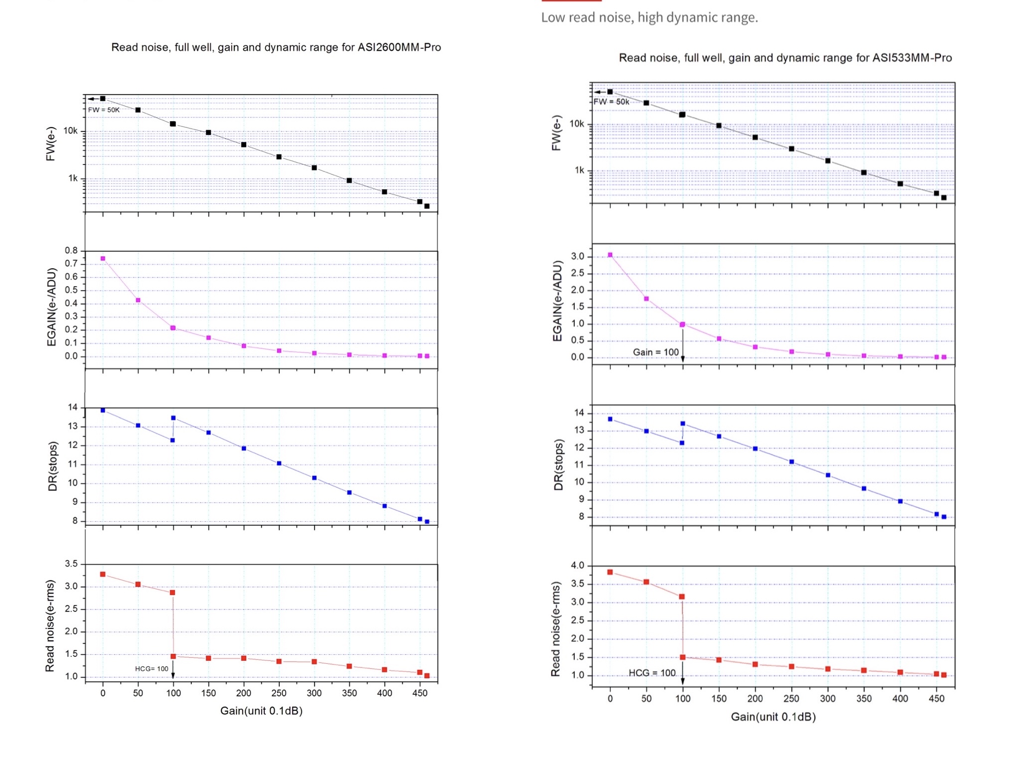
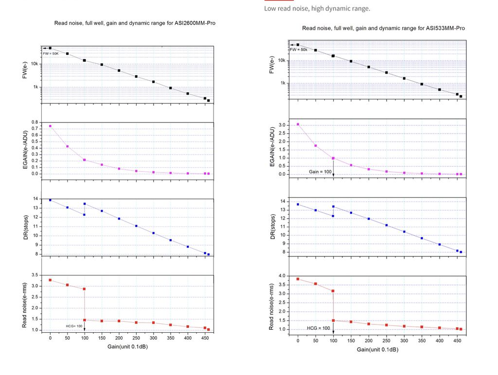
I think the Y axis labelling is incorrect on the 2600 gain curve chart. It show zero electrons per ADU at high gains which is clearly wrong?
Edit: doh it’s because the 2600 has 16bit and 533 has 14bit ADC
|
You cannot like this item. Reason: "ANONYMOUS".
You cannot remove your like from this item.
Editing a post is only allowed within 24 hours after creating it.
You cannot Like this post because the topic is closed.
Copy the URL below to share a direct link to this post.
This post cannot be edited using the classic forums editor.
To edit this post, please enable the "New forums experience" in your settings.
Looks to me like a very sneaky way to hide the real sensor performance. I used a plotdigitze to extract the values and add them into the same graph. I also calculated the ratio as (533/2600). This ratio gets quite errorneous towards higher gain values due to the very small values for both. But looks like the ratio is around 3.5 to 4, almost constant over the whole gain region. 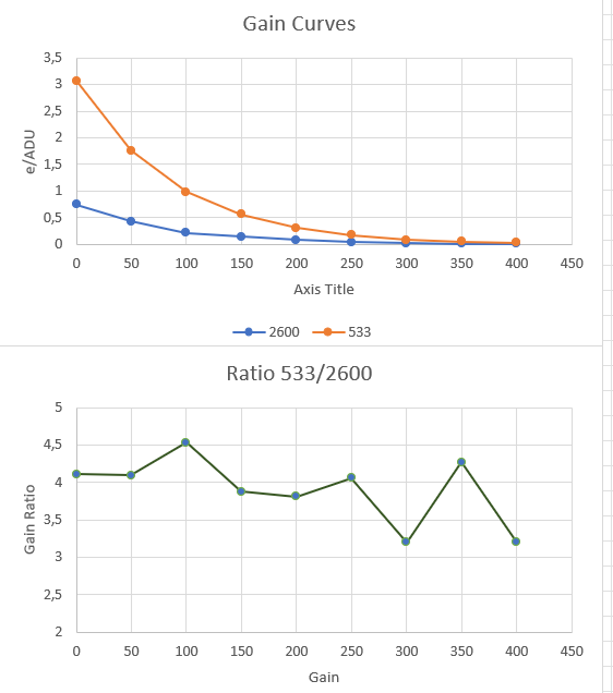 |
You cannot like this item. Reason: "ANONYMOUS".
You cannot remove your like from this item.
Editing a post is only allowed within 24 hours after creating it.
You cannot Like this post because the topic is closed.
Copy the URL below to share a direct link to this post.
This post cannot be edited using the classic forums editor.
To edit this post, please enable the "New forums experience" in your settings.
D. Jung:
Looks to me like a very sneaky way to hide the real sensor performance. I used a plotdigitze to extract the values and add them into the same graph. I also calculated the ratio as (533/2600). This ratio gets quite errorneous towards higher gain values due to the very small values for both. But looks like the ratio is around 3.5 to 4, almost constant over the whole gain region. There is nothing sneaky going on here... the533MM has a 14 bit ADC, the 2600MM has 16 bit. It is natural that you would need to use coarser discretization with the 533MM. This simply adds a bit of quantization noise, which is only meaningful at low gains. It is probably the exact reason why the 533MM has a higher overall noise at Gain 0 than the 2600MM by a small amount - it is the effect of quantization added to the read noise due to the smaller bit depth. At higher gains, because the signal (and the associated read noise) is amplified well above the quantization threshold, the 14 bit vs 16 bit difference does not matter; the quantization noise becomes small compared to other sources of noise. This is why, at high gains, both cameras show near identical dynamic range and noise. This is covered nicely here, in this old but still very relevant publication. https://homes.psd.uchicago.edu/~ejmartin/pix/20d/tests/noise/noise-p3.html#bitdepth |
You cannot like this item. Reason: "ANONYMOUS".
You cannot remove your like from this item.
Editing a post is only allowed within 24 hours after creating it.
You cannot Like this post because the topic is closed.
Copy the URL below to share a direct link to this post.
This post cannot be edited using the classic forums editor.
To edit this post, please enable the "New forums experience" in your settings.
What is the conclusion?
I really want to see a comparison of mono and OSC IMX571 under Bortle 9 for RGB only, mainly stars, because i am thinking about using a color camera for stars only, while mono for everything else.
|
You cannot like this item. Reason: "ANONYMOUS".
You cannot remove your like from this item.
Editing a post is only allowed within 24 hours after creating it.
You cannot Like this post because the topic is closed.
Copy the URL below to share a direct link to this post.
This post cannot be edited using the classic forums editor.
To edit this post, please enable the "New forums experience" in your settings.
Tareq Abdulla:
What is the conclusion?
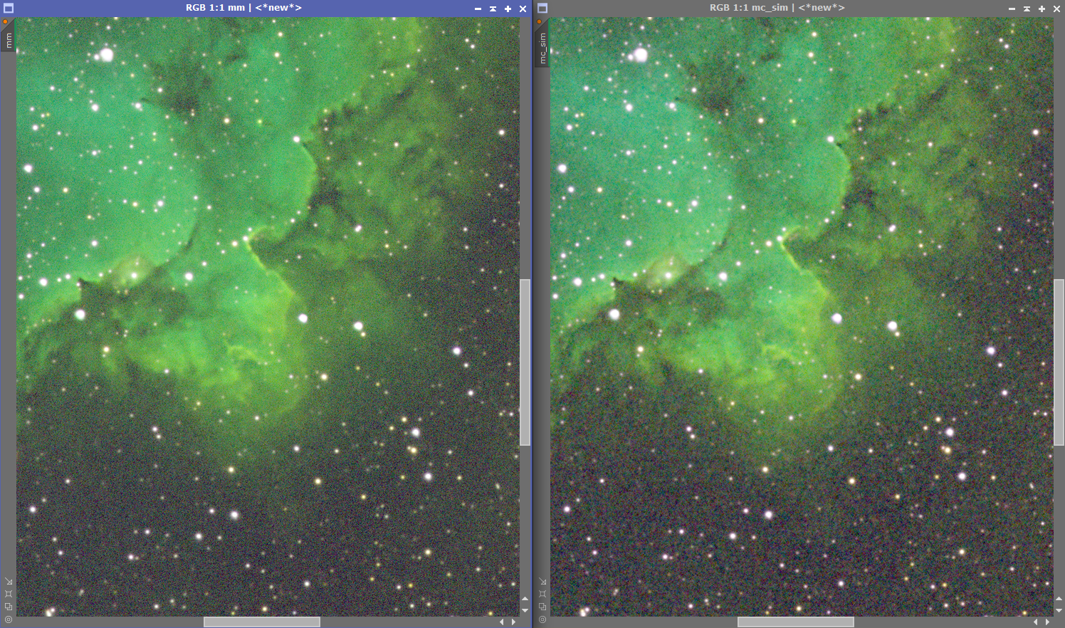
I really want to see a comparison of mono and OSC IMX571 under Bortle 9 for RGB only, mainly stars, because i am thinking about using a color camera for stars only, while mono for everything else. The conclusion is that the 533MC seems about 4 times less sensitive looking at the e/ADU gain curve, which seems to match the hugely different SNR observed. For the comparison between the 2600mm and mc, mayby someone here has both and can post a comparison? For those, the gain curves are identical and the major degrading factors for the MC version should be the debayer process itself, the reduced transmission of the Bayer matrix and the loss of resolution, especially along the diagonals due to the reduced Nyquist frequency (and yes, this can be recovered with drizzle integration, given that you have plenty of clear sky time). I can only simulate a comparison for SHO with the data I have. For simulating the impact of the Bayermatrix, each sub is debayered before integration. This should be a good approximation, as the VNG debayer method is channel independent. For this comparison I assume that the MC has a 85% transmission Bayer matrix, so i use 105min for mono and 2x45=90 min for the MC simulation. Mono, left (total of 105min): 7xHa = 7*5=35min 7xOiii = 7*5=35min 7xSii = 7*5=35min MC simulated, right (total of 90min, 85% of 105min): Ha/Oiii dual (45min): 9xHa = 9*5 = 45min --> r channel used for SHO 9xOiii = 9*5 = 45min --> g channel used for SHO Sii (45min): 9xSii = 9*5 = 45min --> r channel used for SHO I ran BXT over both images, not other image processing applied. 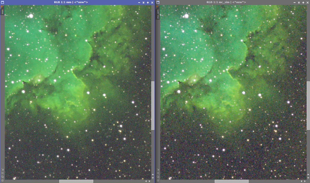 Will be interesting to see if someone with both cameras can confirm or reject this result with real data for both cameras.
|
You cannot like this item. Reason: "ANONYMOUS".
You cannot remove your like from this item.
Editing a post is only allowed within 24 hours after creating it.
You cannot Like this post because the topic is closed.
Copy the URL below to share a direct link to this post.
This post cannot be edited using the classic forums editor.
To edit this post, please enable the "New forums experience" in your settings.
I would disagree with the statement about sensitivity above - there isn’t a benefit to discretizing noise as shown in the Martinec article linked., other than possibly at very low gains. It is a bit like using a very fine ruler to measure length, when the length itself is varying much more than the gradations in the ruler. So it is incorrect to say that the 533 is 3x less sensitive than the 2600 based on the data presented.
All this said - the 2600 certainly offers other advantages like a much bigger sensor area. And certainly a 16 it ADC may not help but it does not hurt either other than in added cost. If you can handle the extra cost and have a scope and processing power to deal with the larger files, you are unlikely to make a mistake going with the 2600.
|
You cannot like this item. Reason: "ANONYMOUS".
You cannot remove your like from this item.
Editing a post is only allowed within 24 hours after creating it.
You cannot Like this post because the topic is closed.
Copy the URL below to share a direct link to this post.
This post cannot be edited using the classic forums editor.
To edit this post, please enable the "New forums experience" in your settings.
Arun H:
I would disagree with the statement about sensitivity above - there isn’t a benefit to discretizing noise as shown in the Martinec article linked., other than possibly at very low gains. It is a bit like using a very fine ruler to measure length, when the length itself is varying much more than the gradations in the ruler. So it is incorrect to say that the 533 is 3x less sensitive than the 2600 based on the data presented.
All this said - the 2600 certainly offers other advantages like a much bigger sensor area. And certainly a 16 it ADC may not help but it does not hurt either other than in added cost. If you can handle the extra cost and have a scope and processing power to deal with the larger files, you are unlikely to make a mistake going with the 2600. Based on the gain curve, the 533 requires 4x as many electrons per ADU. Since the QE is basically the same between both sensors, doesn't that mean you need 4 times as many photons to trigger the same digital signal, hence having a 4 times less sensitive sensor?
|
You cannot like this item. Reason: "ANONYMOUS".
You cannot remove your like from this item.
Editing a post is only allowed within 24 hours after creating it.
You cannot Like this post because the topic is closed.
Copy the URL below to share a direct link to this post.
This post cannot be edited using the classic forums editor.
To edit this post, please enable the "New forums experience" in your settings.
D. Jung:
Since the QE is basically the same between both sensors, doesn't that mean you need 4 times as many photons to trigger the same digital signal, hence having a 4 times less sensitive sensor? If the sensor were truly noiseless, yes, then a 16 bit versus 14 bit ADC would result in a meaningful difference given the available full well capacity. But if you look at the sensor of the 2600MM, the baseline read noise is ~3 electrons. The number three needs two bits to store (11 in binary). That means, the bottom two bits in the 2600 are basically storing noise, and that is at gain 0. And you can actually see this in the graphs presented. The finer discretization of the signal yields a marginal benefit at low gains (at gain 0 specifically) and no benefit at high gains. The quantization noise is being added in quadrature to the read noise. At high gains, what is happening is that the read noise is being amplified well above the 3 electron quantization noise, and 14 bits are more than sufficient to store all the meaningful information that exists. That is why those two curves show no difference in read noise at high gains, and no difference in DR. In the real world, you would have other sources of noise, such as dark current noise and photon shot noise that would render the difference even less meaningful.
|
You cannot like this item. Reason: "ANONYMOUS".
You cannot remove your like from this item.
Editing a post is only allowed within 24 hours after creating it.
You cannot Like this post because the topic is closed.
Copy the URL below to share a direct link to this post.
This post cannot be edited using the classic forums editor.
To edit this post, please enable the "New forums experience" in your settings.
I wanted to add a bit more detail on how quantization error works.
A 14 versus 16 bit ADC does NOT mean that you need 4x the number of electrons with the 14 bit as with the 16 bit. The only thing that's changing is the precision with which digital data is stored.
Restricting to Gain 0 - both the 533 and 2600 have full well capacities of 50,000 e- roughly. To make my point, let us assume that the top end is 49,999 electrons. That number, in binary, is 1100001101001111, which takes 16 bits to store. The 2600's ADC can handle this, but the 533's cannot. So the 533 in essence chops off the bottom two bits to get the number 11000011010011 which is 14 bits. But, note that, in post you can simply add two zeros at the end to get 1100001101001100 which is the number 49996.
So the 2600 can tell the difference between 49996 and 49999 and the 533 cannot, but that difference of 3 electrons is basically lost in the read noise, and becomes even more irrelevant at higher gains or in the presence of other sources of noise.
So, it is incorrect to say that it takes 3-4x the number of electrons to trigger a change. Both sensors at a basic level have the same sensitivity, but the digital data is stored with more precision in the 2600. But, as shown above, that precision is largely irrelevant in most real world cases. As another example, consider the 1600MM Pro, which has only a 12 bit ADC. If it really was that the ASI2600 was 16 times more sensitive than the 1600, we would have been able to shorten our integration times by a factor of 16. That's clearly not the case!
|
You cannot like this item. Reason: "ANONYMOUS".
You cannot remove your like from this item.
Editing a post is only allowed within 24 hours after creating it.
You cannot Like this post because the topic is closed.
Copy the URL below to share a direct link to this post.
This post cannot be edited using the classic forums editor.
To edit this post, please enable the "New forums experience" in your settings.
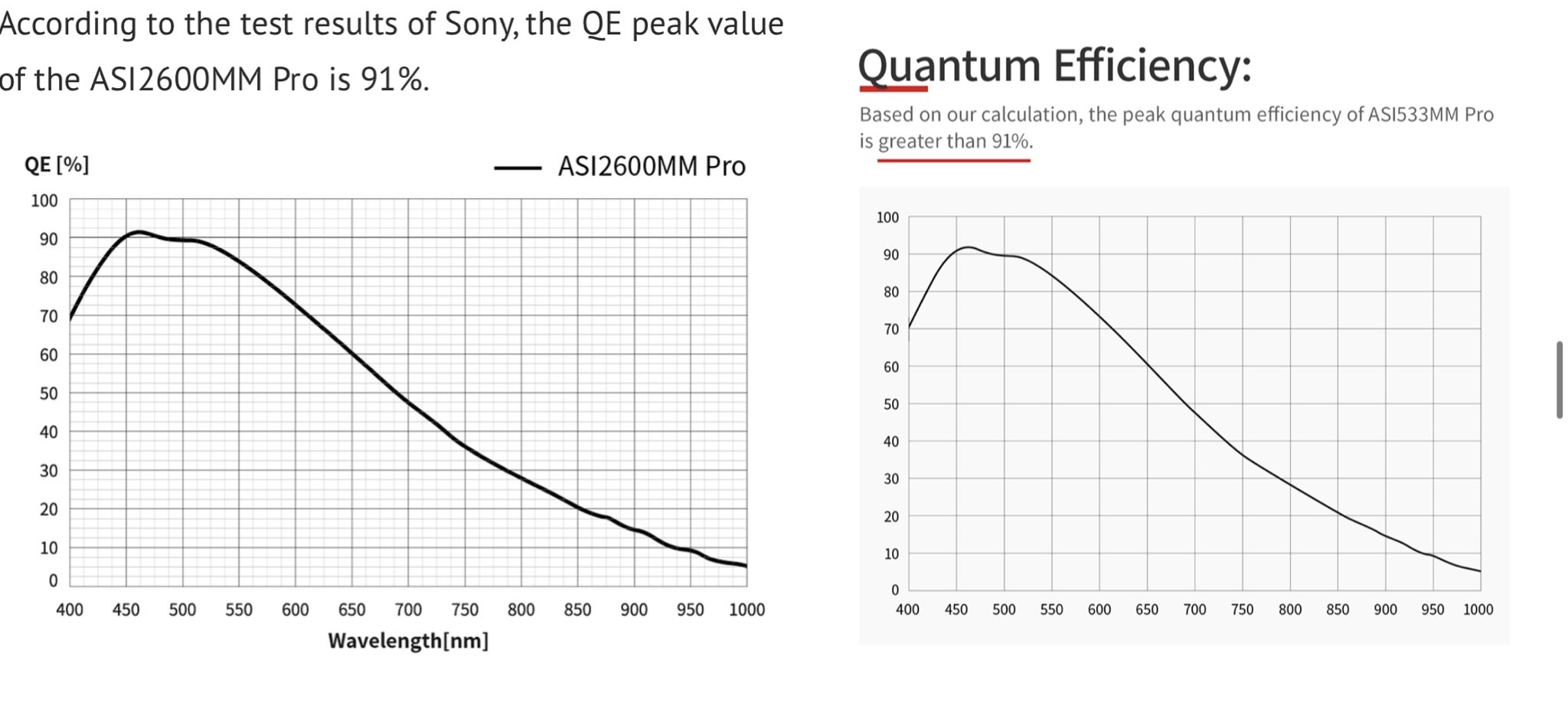
So how does the Bayer array effect actual QE. My understanding that QE is measured without the filters in place. That would explain how both sensors can be exactly the same in that regard.
|
You cannot like this item. Reason: "ANONYMOUS".
You cannot remove your like from this item.
Editing a post is only allowed within 24 hours after creating it.
You cannot Like this post because the topic is closed.
Copy the URL below to share a direct link to this post.
This post cannot be edited using the classic forums editor.
To edit this post, please enable the "New forums experience" in your settings.
Tony Gondola:
So how does the Bayer array effect actual QE. My understanding that QE is measured without the filters in place. That would explain how both sensors can be exactly the same in that regard. take a look at ZWO’s page on the 533 for example. There are two curves - one for the sensor alone and one which is basically %T vs wavelength for each of the Bayer array colors. You simply take the mono curve and multiply it by the efficiency of the particular Bayer array color you are interested in. That is how they come up with a peak efficiency of 90% for mono and 80% for color. They are reporting the maximum efficiency achieved in color - which is for the green filter around 500nm which has an %T of 90% and where the base mono efficiency is 90%. The product of those two numbers is your net peak efficiency for the MC: https://www.zwoastro.com/product/asi533-pro-series/ |
You cannot like this item. Reason: "ANONYMOUS".
You cannot remove your like from this item.
Editing a post is only allowed within 24 hours after creating it.
You cannot Like this post because the topic is closed.
Copy the URL below to share a direct link to this post.
This post cannot be edited using the classic forums editor.
To edit this post, please enable the "New forums experience" in your settings.
Tony Gondola:
So how does the Bayer array effect actual QE. My understanding that QE is measured without the filters in place. That would explain how both sensors can be exactly the same in that regard. In my opinion, QE is one of the most overemphasised, misunderstood and largely irrelevant measurements people use to justify a camera purchase. In the past 24 months I've used a KAF-8300M, IMX294, Panasonic MN34230, and IMX571M Despite the IMX294 (even with being colour) having a higher QE than the 1600MM, the 1600MM created a FAR brighter image in less integration time than the 294C. The 1600MM and KAF8300M have similar QE characteristics, (The 1600MM had a higher peak QE, but the KAF8300M had higher QE where it mattered) Neither were noticably brighter than the other for a given integration time. (noise was the separating factor, but not QE). The IMX571 mono has a peak QE that is MUCH higher than either the 1600MM or the KAF8300M, and in luminance images, I think I can tell... but it may be just that its far less noisy than either of those cameras.. but with a Ha filter in front of it - the 1600MM and the KAF8300M both match it quite easily, because the QE of that 571 peaks and the blue/green end of the spectrum, and the KAF8300 is JUUUUUUST about as sensitive at 656.3nm... again, there's a noise difference... Does QE matter... Sure.. I guess.. Should QE be considered closely when buying a new camera? No... not really... The ONE place I'll say I've seen a big difference is between the KAF8300 and IMX571 when shooting OIII data. OIII is captured far more quickly on the 571.
|
You cannot like this item. Reason: "ANONYMOUS".
You cannot remove your like from this item.
Editing a post is only allowed within 24 hours after creating it.
You cannot Like this post because the topic is closed.
Copy the URL below to share a direct link to this post.
This post cannot be edited using the classic forums editor.
To edit this post, please enable the "New forums experience" in your settings.
Arun H:
Tony Gondola:
So how does the Bayer array effect actual QE. My understanding that QE is measured without the filters in place. That would explain how both sensors can be exactly the same in that regard.
take a look at ZWO’s page on the 533 for example. There are two curves - one for the sensor alone and one which is basically %T vs wavelength for each of the Bayer array colors. You simply take the mono curve and multiply it by the efficiency of the particular Bayer array color you are interested in. That is how they come up with a peak efficiency of 90% for mono and 80% for color. They are reporting the maximum efficiency achieved in color - which is for the green filter around 500nm which has an %T of 90% and where the base mono efficiency is 90%. The product of those two numbers is your net peak efficiency for the MC:
https://www.zwoastro.com/product/asi533-pro-series/ ZWO isn't the place to look for this sort of things... "we believe that..." that sort of crap. 90% QE? Gimme a break... (not you Arun, them).
|
You cannot like this item. Reason: "ANONYMOUS".
You cannot remove your like from this item.
Editing a post is only allowed within 24 hours after creating it.
You cannot Like this post because the topic is closed.
Copy the URL below to share a direct link to this post.
This post cannot be edited using the classic forums editor.
To edit this post, please enable the "New forums experience" in your settings.